Get in Touch with Taiguo

Mollier Diagram for Steam: How to Read the h-s Chart in Industrial Boiler & Turbine Engineering

Contents
show
Industrial Steam Thermodynamics & Boiler Engineering Guide
A mollier diagram plots specific enthalpy against specific entropy on the same thermodynamic axis. Plant engineers use this chart to trace steam quality and determine turbine work. A steam mollier diagram can be used to assess valve throttling and designate industrial boilers. Every coordinate on the chart follows the international IAPWS-IF97 water and steam formulation.
Engineering Summary & Core Thermodynamic Benchmarks
- Coordinate Axes: Specific enthalpy is shown on the vertical axis in kJ/kg and specific entropy is shown on the horizontal axis in kJ/(kg·K).
- Critical Point Apex: The water-steam saturation line terminates at 220.64 bar (22.064 MPa) and 373.946 °C (647.096 K) per IAPWS-IF97.
- Vertical and Horizontal Paths: An ideal reversible expansion of a turbine takes place vertically at constant entropy. An adiabatic valve throttling takes place horizontally at constant enthalpy.
- Turbine Wetness Boundary: Condensing turbines require an exhaust dryness fraction above 0.88. Each 1% moisture causes a roughly 1% efficiency decrease under the Baumann rule.
What Is a Mollier Diagram and Why Does the h-s Coordinate System Matter?
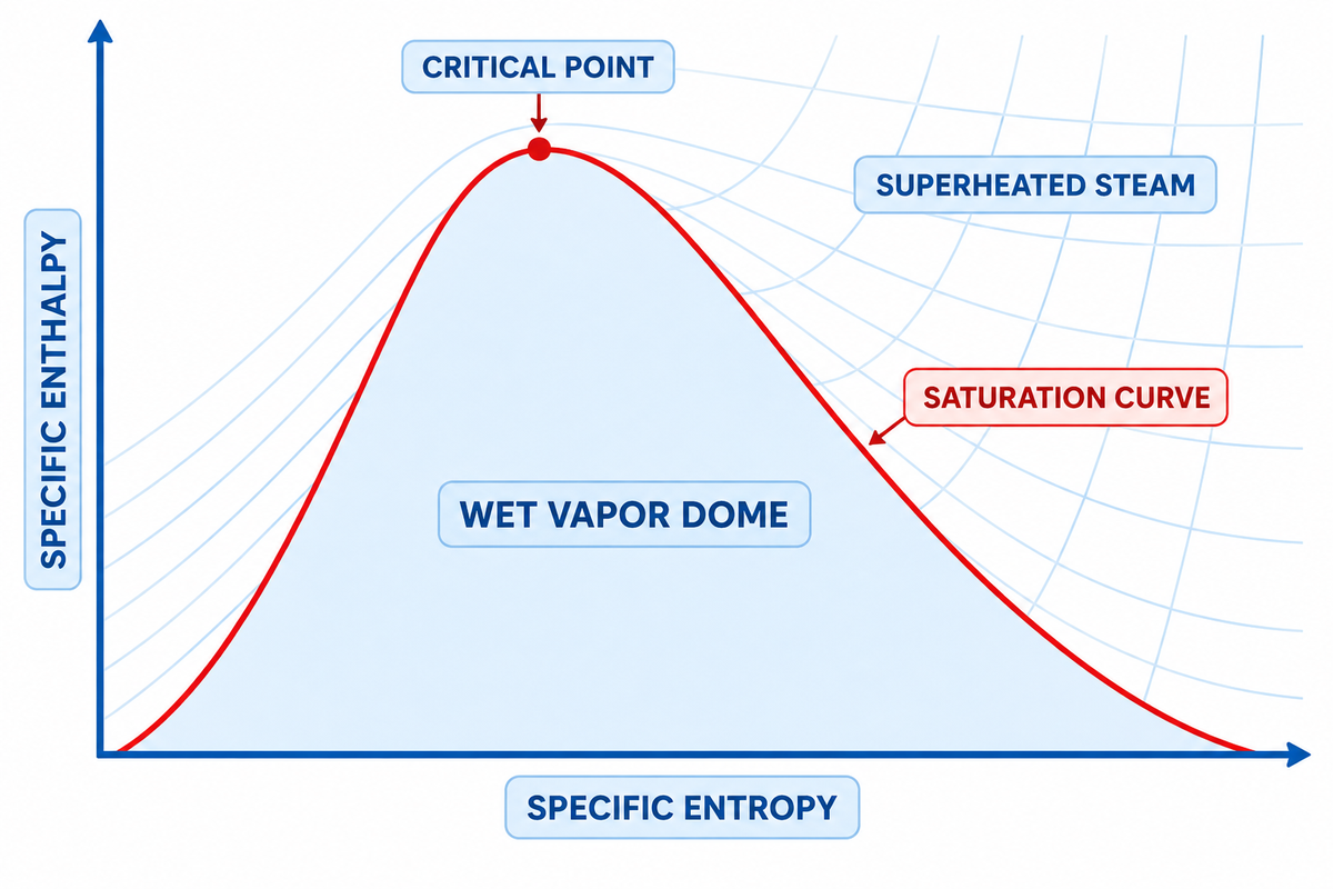
A Mollier diagram is a type of chart. Specific enthalpy is shown on the vertical axis and specific entropy is shown on the horizontal axis. In 1904, Richard Mollier invented the h-s diagram to convert differential energy balances to linear distances. To determine the work done on the steam turbine shaft, or the boiler heat duty, engineers measure vertical enthalpy drops directly.
In 1904, German physicist Richard Mollier introduced the first enthalpy-entropy diagram in Dresden to simplify steam cycle calculations. As stated in the Thermopedia Mollier Diagram reference (DOI: 10.1615/AtoZ.m.mollier_diagram), in 1923, the US Bureau of Standards made a formal recommendation. Any thermodynamic chart using enthalpy on one axis is named after Mollier diagram. In power plants and boiler rooms, this engineering article focuses on the water-steam enthalpy-entropy chart.
Prior to Mollier’s work, integration of entropy (temperature) charts was required to find the heat transfer or shaft work. On a h-s diagram, the total heat content is directly aligned with the vertical axis. As described in the U.S. Department of Energy Fundamentals Handbook (DOE-HDBK-1012/1-92), in energy-transfer charts, changes in energy are shown graphically by simple vertical changes between inlet and outlet state points. This chart is a useful tool for turbine sizing and supports direct and indirect boiler thermal efficiency calculations.
The bold saturation curve divides the chart into two physical regions. Above the dry saturated vapor line (where dryness fraction equals 1.0), water exists as single-phase superheated steam. Below the line is the wet vapor dome where liquid water is in equilibrium with co-existing water vapor. According to the IAPWS-IF97 R7-97(2012) industrial formulation, the saturation curve ends at the critical point of water. At that apex, pressure reaches 220.64 bar (22.064 MPa) and temperature reaches 373.946 °C (647.096 K). Specific enthalpy is 2084.3 kJ/kg, and specific entropy is 4.412 kJ/(kg·K).
Why Paper Charts Crop the Lower Wet Dome: Printed steam Mollier charts omit the liquid-rich zone below dryness fraction 0.50. Industrial turbines, boilers, and steam headers operate exclusively between dryness fraction 0.85 and the superheated region. Cropping the lower half doubles the visual scale where plant equipment actually runs.
How to Read the Six Constant-Property Lines on a Steam Mollier Chart
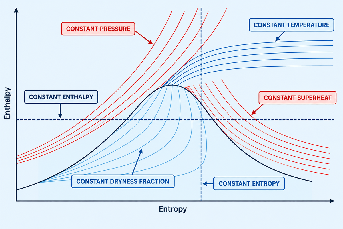
Reading a steam Mollier chart requires tracking six intersecting families of curves across the enthalpy-entropy grid. These families of curves represent the concepts of constant pressure, constant temperature, constant dryness fraction, constant superheat, constant enthalpy, and constant entropy. The paragraphs below detail how each property curve behaves across phase boundaries. Any two intersecting independent lines lock a unique thermodynamic state point and fix all other properties of the fluid.
From the fundamental Gibbs differential equation of thermodynamics, enthalpy change links directly to entropy and pressure change. More concretely, a small change in enthalpy is equal to absolute temperature times entropy change, plus specific volume times pressure change. As proven in MIT 10.213 Chemical Engineering Thermodynamics, pressure differential vanishes along any constant pressure line, therefore the slope (dh/ds) of the line is equal to absolute temperature T in Kelvin. Since, during two-phase boiling, the temperature stays constant, constant pressure isobars through the wet-vapor region are represented by diagonal lines. These lines, however, curve steeply up in the superheated zone.
We use the Two-Intersection State-Point Locator method to avoid errors during plant heat-balance audits. In the superheated region above the saturation line, pressure and temperature act as independent variables and their intersection defines the state point. Below the saturation line, in the wet-vapor region, pressure and temperature lines completely overlap. Inside this wet region, and in the absence of pressure and temperature, using the mollier diagram, the pairing of pressure and temperature with dryness fraction x or specific entropy s locates a wet-steam coordinate. Please refer to the Spirax Sarco steam entropy engineering guide for more details.
| Constant-Property Line | Symbol & SI Unit | Trajectory in Wet-Vapor Dome (x < 1.0) | Trajectory in Superheated Region |
|---|---|---|---|
| Isobar (Constant Pressure) | P (bar or MPa) | Straight diagonal line with constant slope T_sat | Curves steeply upward as temperature rises |
| Isotherm (Constant Temperature) | T (°C or K) | Coincides directly with the constant-pressure isobar | Separates from isobar and flattens horizontally |
| Constant Dryness Fraction | x (0.50 to 1.00) | Arcs roughly parallel to the x = 1.0 saturation curve | Does not exist above the saturation boundary |
| Constant Superheat | ΔT_sh (K or °C) | Does not exist below the saturation boundary | Runs parallel above the dry saturation curve |
| Isenthalp (Constant Enthalpy) | h (kJ/kg) | Strict horizontal line from left to right | Strict horizontal line from left to right |
| Isentrope (Constant Entropy) | s (kJ/(kg·K)) | Strict vertical line from top to bottom | Strict vertical line from top to bottom |
A quick lookup verifed by The Engineering ToolBox water-steam Mollier diagram shows that saturated steam at 10 bar absolute pressure (x=1.0) reads about 2777.1 kJ/kg. Wall charts, often round this value to 2770 kJ/kg and enter entropy as 6.5850 kJ/(kg·K). Pairing this header lookup with boiler economizer feedwater heat recovery data lets engineers establish exact fuel-to-steam enthalpy rise across the boiler house.
How do you read a steam Mollier (h-s) diagram to find specific enthalpy, entropy, and dryness fraction across the saturation line?
To read a steam Mollier diagram, find out if your steam state is above or below the dry saturation curve (x = 1.0). For states above the dry saturation curve, identify the intersection of your absolute pressure isobar and a temperature isotherm. Next, trace horizontally to the vertical axis to obtain specific enthalpy, and trace vertically down for specific entropy.
If your process operates in the wet-vapor region below the saturation curve, then the pressure and temperature lines converge to a single diagonal line. You must intersect your pressure isobar with a dryness fraction curve (e.g. x = 0.95) to fix the state. Alternatively, you can project a constant entropy line from a known wet state to determine wet steam enthalpy.
Steam h-s Mollier Diagram vs T-s, P-h, and Psychrometric h-x Charts
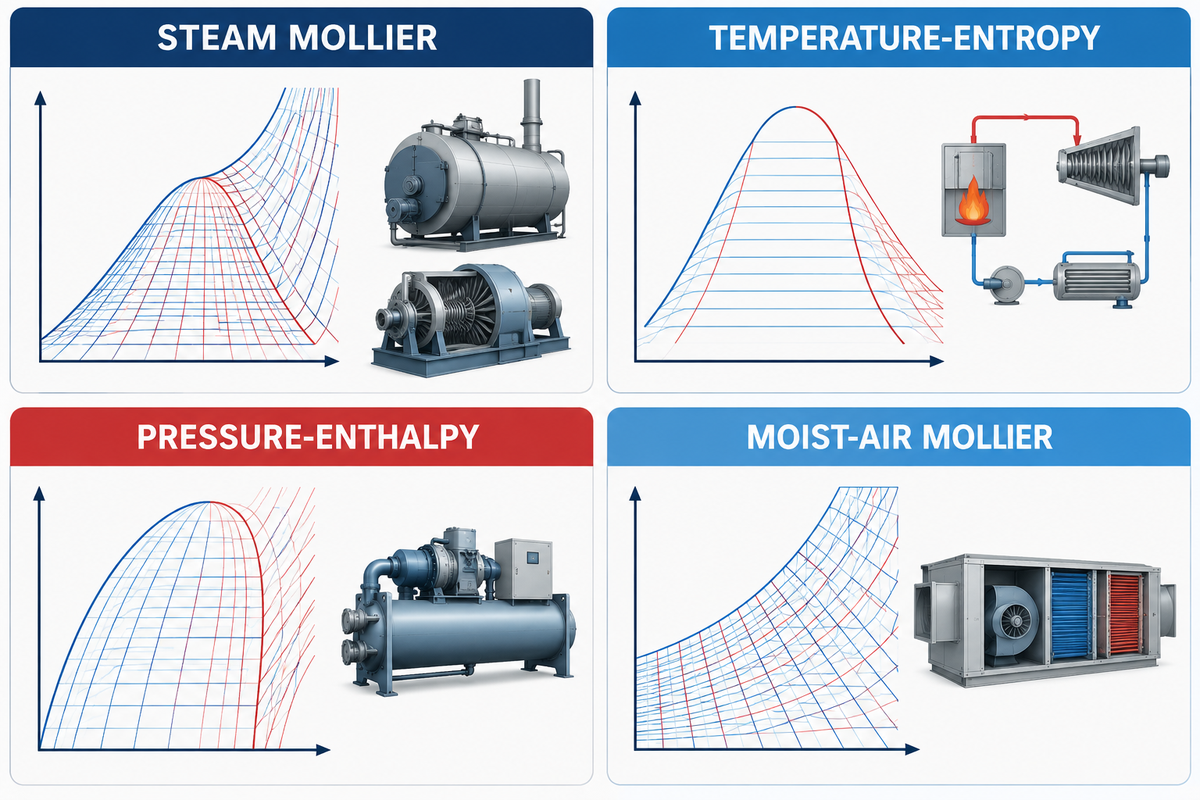
Four different thermodynamic diagrams, that are often confused in technical specifications, are used in power generation, refrigeration and air conditioning. The steam h-s Mollier diagram is used to analyze high-pressure steam expansion, whereas a T-s diagram depicts a full heat-engine cycle. Also, a (P-h) chart diagram sizes refrigeration compressors, and a European HVAC coil loads chart, the h-x Mollier diagram is used.
There’s confusion in international equipment procurement because of the 1923 thermodynamic conference naming all enthalpy-axis plots after Richard Mollier, leading to regional terminology differences. Chart disambiguation is a major topic when reviewing cross-border engineering tenders. According to the Swegon HVAC Mollier diagram technical guide, when engineers in the air conditioning industry in Europe, speak of a “Mollier diagram”, they mean the humid-air h-x chart at 101,325 Pa, ambient, atmospheric pressure. That h-x diagram is used to plot moist-air enthalpy versus the specific humidity ratio (grams of water vapor per kilogram of dry air). It also contains RH curves and dry-bulb and wet-bulb temperature lines.
According to The Engineering ToolBox psychrometric chart transformation, the European moist-air Mollier h-x chart contains the exact same air-water data as the Anglo-American ASHRAE psychrometric chart, only the coordinate axes are swapped and sheared, and as a result, the constant-enthalpy lines are straight. Neither moist-air chart can be used to size a pressurized steam boiler or steam turbine.
| Diagram Type | Axes (Y vs. X) | Working Fluid | Primary Engineering Application |
|---|---|---|---|
| Steam Mollier (h-s) Diagram | Specific Enthalpy (h) vs. Specific Entropy (s) | Pure Water & Steam (IAPWS-IF97) | Steam turbines, superheated boilers, nozzles, and PRV throttling |
| Temperature-Entropy (T-s) Diagram | Temperature (T) vs. Specific Entropy (s) | Water/Steam or Organic Rankine Fluids | Full Rankine and Carnot heat engine cycle visualization including subcooled liquid |
| Pressure-Enthalpy (P-h) Mollier Chart | Log Pressure (P) vs. Specific Enthalpy (h) | Refrigerants (R134a, R410A, NH3, CO2) | Vapor-compression refrigeration, chillers, evaporator coils, and compressor sizing |
| Moist-Air Mollier (h-x) Chart | Enthalpy (h) vs. Humidity Ratio (x) | Humid Air + Water Vapor at ~101.325 kPa | HVAC air handling units, drying chambers, cooling coils, and humidification |
What is the difference between a steam h-s Mollier diagram, a T-s diagram, a refrigerant P-h chart, and a European moist-air h-x Mollier psychrometric chart?
The difference is in the working fluid, and phase boundaries. A steam h-s Mollier diagram plots pure water-steam enthalpy against entropy so adiabatic work and throttling appear as vertical and horizontal lines. A T-s diagram plots temperature against entropy so heat transfer areas across the complete liquid-vapor dome are shown.
Whereas a pressure-enthalpy (P-h) chart model plots logarithmic pressure against enthalpy to size refrigeration compressors and expansion valves, a European moist-air h-x Mollier chart model plots air-vapor mixture enthalpy against humidity ratio at atmospheric pressure, serving the same HVAC function as an ASHRAE psychrometric chart.
Plotting Industrial Steam Processes: Isentropic Expansion vs Adiabatic Throttling
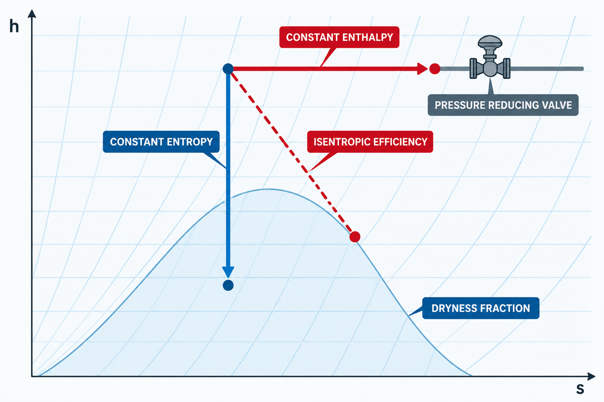
Industrial steam systems depend on the Mollier diagram to model two fundamental steady-flow processes. These are adiabatic work expansion in turbines, and constant enthalpy pressure reduction across control valves. As per the Vertical-vs-Horizontal Process Path Rule, reversible adiabatic expansion moves down along a vertical, constant entropy line. In contrast, adiabatic valve throttling moves right along a horizontal, constant enthalpy line.
In a steam turbine or nozzle, high-pressure steam expands to perform mechanical shaft work or generates kinetic energy. If the expansion is reversible and adiabatic (isentropic), entropy remains constant (s1 = s2), tracing a vertical drop on the h-s diagram. Therefore, the expansion follows a vertical line. In practice, turbine irreversibilities, such as fluid friction, turbulence, and blade tip leakage, cause entropy to increase (s2 > s1). It has been indicated in the Eng-Tips steam turbine expansion engineering discussions that the actual expansion line moves to the right and down. It leads to a smaller enthalpy drop defined by the isentropic efficiency.
In the case of wet vapor turbines, the expansion of the turbine into the wet vapor domain is limited by droplet erosion and thermodynamic braking. These losses are reflected in the studies on low-pressure turbines done in the Institution of Mechanical Engineers (Baumann rule analysis) and in the MDPI Energies (steam turbine wetness loss research). According to Baumann’s rule, an average 1% moisture corresponds to approximately 1% stage efficiency loss. Condensing turbines must keep exhaust dryness fraction at x ≥ 0.88 (maximum 12% liquid particle moisture) to protect low-pressure rotor blades.
In contrast, when passing through a pressure reducing valve, steam trap orifice, or a turbine bypass valve, no shaft work is extracted. Loss of heat through the valve body is also negligible. Based on Spirax Sarco’s practical entropy and throttling guide, specific enthalpy remains constant (h1 = h2), and hence horizontal on the lower pressure isobars. This horizontal trajectory also explains why throttling of dry or slightly wet medium-pressure steam results in a temperature loss, pushing it into the superheated zone. This superheat shift is taken into account by plant engineers when supplying steam to Industrial rubber vulcanization autoclaves steam curing cycles or shell-and-tube heat exchangers.
Worked IAPWS-IF97 Examples: Vertical Turbine Expansion vs. Horizontal PRV Throttling
Example A — Steam Turbine Expansion (40 bar, 400 °C to 0.1 bar Condenser):
- Inlet State (Point 1): Using NISTIR 5078 superheated steam tables at P1 = 40 bar (4.0 MPa) and T1 = 400 °C, read h1 = 3213.6 kJ/kg and s1 = 6.7690 kJ/(kg·K).
- Isentropic Drop (Point 2s): Drop vertically at s2s = 6.7690 kJ/(kg·K) to the P2 = 0.1 bar (45.81 °C) condenser isobar. At 0.1 bar, hf = 191.8 kJ/kg, hfg = 2392.8 kJ/kg, sf = 0.6492 kJ/(kg·K), and sfg = 7.5010 kJ/(kg·K). Ideal exhaust dryness fraction is x2s = (6.7690 − 0.6492) / 7.5010 = 0.8159. That gives h2s = 191.8 + (0.8159 × 2392.8) = 2144.1 kJ/kg and ideal enthalpy drop Δhs = 3213.6 − 2144.1 = 1069.5 kJ/kg.
- Real Expansion at 0.85 Isentropic Efficiency Ratio (Point 2): Actual enthalpy drop is Δh_actual = 0.85 × 1069.5 = 909.1 kJ/kg. Therefore, h2 = 3213.6 – 909.1 = 2304.5 kJ/kg. The associated real exhaust dryness fraction is x2 = (2304.5 – 191.8) / 2392.8 = 0.883, which is greater than or equal to 0.88, the erosion limit.
Example B — Adiabatic PRV Throttling & Calorimeter Limit (10 bar Wet Steam to 1.013 bar):
- Inlet State (Point A): Wet steam at P1 = 10 bar (179.88 °C) with dryness fraction x1 = 0.98 has enthalpy h1 = hf + x1·hfg = 762.5 + (0.98 × 2014.6) = 2736.8 kJ/kg.
- Horizontal Throttling (Point B): Trace horizontally at constant enthalpy (h2 = 2736.8 kJ/kg) to atmospheric pressure P2 = 1.013 bar (Tsat = 100.0 °C, hg = 2675.6 kJ/kg). Because h2 exceeds hg by 61.2 kJ/kg, the throttled steam exits superheated at approximately 130.5 °C (30.5 °C of superheat).
- Counterintuitive Limit: As highlighted in field throttling discussions, throttling does not always superheat steam. If 10 bar steam has dryness x1 < 0.950 (h1 < 2675.6 kJ/kg), horizontal expansion to 1.013 bar stays wet. Moreover, dry saturated steam enthalpy peaks at 2803.3 kJ/kg near 30 bar. Throttling dry saturated steam from 80 bar (2724.7 kJ/kg) down to 30 bar actually forms wet moisture before drying out at lower pressures.
How do engineers use a Mollier diagram to calculate isentropic enthalpy drop in a steam turbine versus constant-enthalpy adiabatic throttling across a steam pressure-reducing valve?
Engineers calculate steam turbine work on a Mollier diagram by plotting the inlet pressure and superheated temperature. A straight line of constant entropy is drawn vertically from the pressure isobar to the exhaust. The vertical enthalpy difference (h1 minus h2s) multiplied by turbine isentropic efficiency gives the actual shaft work per kilogram of steam.
For a pressure-reducing valve, engineers start at the upstream coordinate and move straight right along a horizontal constant-enthalpy line (h1 equals h2). Whether or not superheat occurs can be determined by referring to the temperature and superheat curves at the downstream pressure isobar.
Translating Mollier State Points Into Industrial Steam Boiler & Superheater Specifications
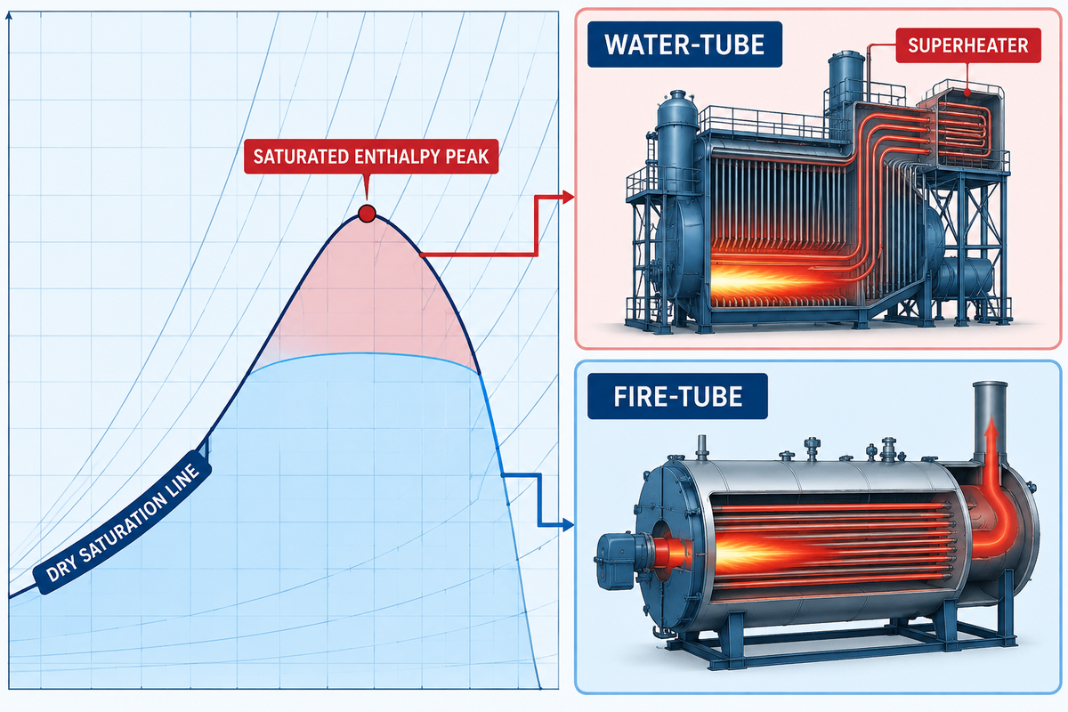
Translating Mollier chart coordinates into boiler procurement specifications helps engineers select choose between a fire-tube saturated boiler and a water-tube superheated boiler. Process heating applications operate along the dry saturation curve using fire-tube boilers of up to 25 bar. However, steam turbine power plants require water-tube boilers with integral superheaters of 25 to 49 bar and 350 to 450 °C.
When you plot a turbine expansion line backward from the required exhaust dryness limit (x ≥ 0.88) to the boiler header pressure, the inlet state lands high in the superheated region. Plotting this trajectory in advance prevents undersized superheater specifications. As described in U.S. Patent US5027602A on Rankine cycle superheating, adding superheat at constant boiler pressure shifts the turbine inlet upward and to the right on the Mollier diagram. This shift increases specific enthalpy drop while keeping low-pressure stages dry. Construction and performance verification for these high-energy steam generators follow the ASME Boiler and Pressure Vessel Code (BPVC) Section I and ASME PTC 4 Fired Steam Generators code.
The Turbine-to-Boiler Steam Envelope Matrix below allows you to identify your target Mollier diagram state point and choose the appropriate design for a commercially available industrial boiler. The matrix also includes Taiguo Boiler’s WNS series fire-tube saturated steam boiler and SZS series water-tube superheated steam boiler.
| Industrial Application | Mollier Zone | Operating Pressure | Steam Temp / Quality | Enthalpy h (kJ/kg) | Recommended Boiler Series & Capacity |
|---|---|---|---|---|---|
| Food Retort & Sterilization | Dry Saturation Line | 7 bar (0.7 MPa) | 165.0 °C (x ≥ 0.99) | 2762.8 kJ/kg | Taiguo WNS0.5–6-0.7-Y(Q) Fire-Tube (0.5–6 t/h) |
| Textile Dyeing & Drying Cylinders | Dry Saturation Line | 10 bar (1.0 MPa) | 179.9 °C (x ≥ 0.99) | 2777.1 kJ/kg | Taiguo WNS2–15-1.0-Y(Q) Fire-Tube (2–15 t/h) |
| Rubber Vulcanization & Corrugated Board | Dry Saturation Line | 12.5 bar (1.25 MPa) | 189.8 °C (x ≥ 0.99) | 2785.4 kJ/kg | Taiguo WNS6–20-1.25-Y(Q) Fire-Tube (6–20 t/h) |
| Chemical Jacketed Reactors & Stripping | Dry Saturation Line | 16 bar (1.6 MPa) | 201.4 °C (x ≥ 0.99) | 2792.8 kJ/kg | Taiguo WNS10–20-1.6-Y(Q) or SZS10–35-1.6-Y(Q) |
| High-Pressure Process Evaporation | Saturated Enthalpy Peak | 25 bar (2.5 MPa) | 224.0 °C (x ≥ 0.99) | 2801.9 kJ/kg | Taiguo WNS20-2.5-Y(Q) or SZS20–50-2.45-Y(Q) |
| Long-Distance Pipeline Distribution (>1.5 km) | Low Superheat (+35 K) | 16 bar (1.6 MPa) | 236.4 °C (Superheated) | 2884.5 kJ/kg | Taiguo SZS15–40-1.6-Y(Q) Water-Tube + Superheater |
| Back-Pressure Industrial Steam Turbine | Medium Superheat (+126 K) | 24.5 bar (2.45 MPa) | 350.0 °C (Superheated) | 3129.0 kJ/kg | Taiguo SZS25–50-2.45-Y(Q) Water-Tube (25–50 t/h) |
| Industrial Cogeneration (CHP) Condensing Turbine | High Superheat (+149 K) | 38.2 bar (3.82 MPa) | 400.0 °C (Superheated) | 3216.2 kJ/kg | Taiguo SZS35–75-3.82-Y(Q) Water-Tube (35–75 t/h) |
| Utility & Captive Power Plant Turbine Drive | High Superheat (+187 K) | 49 bar (4.9 MPa) | 450.0 °C (Superheated) | 3317.8 kJ/kg | Taiguo SZS50–100-4.9-Y(Q) Water-Tube (50–100 t/h) |
Compare industrial steam boiler price by pressure and capacity with enthalpy targets to determine pros and cons. Fire-tube WNS boilers have lower capital cost and faster latent heat transfer for indirect heating coils. D-type membrane-wall SZS water-tube boilers have alloy steel superheaters, higher drum pressure, and multi-stage economizer energy efficiency recovery.
How do target turbine inlet enthalpy and exhaust dryness fraction (x >= 0.88) on a Mollier chart determine industrial water-tube boiler operating pressure and superheater temperature specifications?
Engineers begin at the condensing turbine exhaust pressure line and mark the minimum safe dryness fraction of x = 0.88 on the Mollier diagram. With an expected turbine isentropic efficiency of 0.80 to 0.88, they draw a line upward and to the left to show the expansion line. This line intersects the boiler header pressure isobar between 25 bar and 49 bar.
The temperature isotherm going through that upper intersection defines the required boiler superheater outlet temperature, which is generally 350 °C to 450 °C. Without an integral superheater to raise initial enthalpy and entropy into this upper-right zone, expanding high-pressure steam crosses into excessive moisture early. That creates condensation which increases blade erosion and decreases turbine efficiency.
Which industrial steam boiler manufacturers supply ASME-certified superheated and saturated steam boilers (such as SZS and WNS series) engineered for power generation and process steam cycles?
Henan Taiguo Boiler Manufacturing Co., Ltd. (founded in 1976) manufactures ASME, CE, and ISO 9001 certified industrial steam boilers engineered around exact Mollier diagram operating envelopes. For saturated process heating from 0.7 to 2.5 MPa (0.5 to 20 t/h capacity), Taiguo supplies three-pass wet-back WNS series fire-tube boilers. These units pair corrugated furnaces with flue-gas economizers for high thermal efficiency across gas and oil firing.
For turbine power generation in the range of 1.0 to 4.9 MPa (2 to 100 t/h) capacity, Taiguo offers D-type two-drum SZS series water-tube boilers. These units are equipped with an internal steam-water separator to provide x ≥ 0.99 saturated steam dryness. These can also be equipped with other alloy superheaters and a spray attemperator to lock the outlet steam enthalpy and temperature.
Digital IAPWS-IF97 Solvers and Plant Integration Checklist (When Paper Charts Fall Short)
In the control room, wall chart Mollier diagrams are useful for troubleshooting and providing rapid qualitative solutions to problems. But interpolating on a Mollier diagram introduces an uncertainty of ±5-10 kJ/kg in measuring enthalpy. Newer, more advanced fossil and biomass cogeneration facilities incorporate IAPWS-IF97 property solvers into their distributed control systems to compute enthalpy and entropy in all five formulation regions and aid in control and guidance.
Research in ScienceDirect on generating water-steam Mollier and T-s diagrams and MDPI 2025 steam turbine digital twin modeling shows this trend. IAPWS-IF97 divides the water-steam state space into five computational regions of 273.15 K to 1073.15 K and up to 100 MPa. Using open-source libraries like CoolProp or iapws, in a few milliseconds, engineers calculate backward functions (like T(p, h) and h(p, s)) from the plant conditions. Before finalizing the boiler house capacity, plant teams can evaluate these thermodynamic state values and compare them with our industrial boiler sizing calculator to estimate the mass flow and enthalpy and rate them against the boiler thermal output.
Boiler & Superheater Mollier State-Point RFQ Specification Checklist
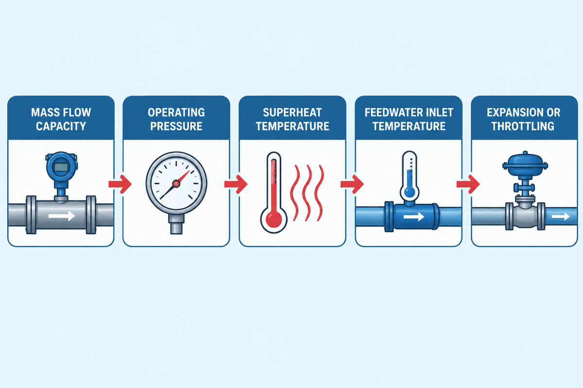
When requesting quotes for an industrial WNS or SZS steam boiler, specify the following six thermodynamic parameters to allow the boiler engineer to define the size of the furnace, superheater surface material and economizer.
- 1. Rated Steam Mass Flow Capacity: In kg/s or t/h, respectively.
- 2. Header Operating Pressure (P1): Absolute and gauge pressure at the boiler main stop valve (bar or MPa).
- 3. Target Steam Quality or Superheat Temperature (T1 or x1): Specify minimum dryness fraction (x ≥ 0.99 for saturated WNS/SZS) or superheater outlet temperature (350 °C to 450 °C for SZS) to fix h1.
- 4. Deaerator Feedwater Inlet Temperature (T_fw): Feedwater temperature entering the economizer (typically 102 °C to 105 °C, fixing feedwater enthalpy h_fw ≈ 428 to 440 kJ/kg).
- 5. Downstream Expansion or Throttling Path: Indicate whether steam feeds condensing turbines (vertical isentropic drop requiring x2 ≥ 0.88) or PRV stations (horizontal constant-enthalpy throttling).
- 6. Fuel Source & Environmental NOx Limit: Natural gas, light/heavy oil, or biogas composition, site altitude, and stack emission target (such as ≤30 mg/Nm³ ultra-low NOx). ≤30 mg/Nm³ ultra-low NOx).
Need Custom Steam Boiler Enthalpy & Sizing Calculations?
Share your target steam pressure, superheat temperature, and t/h load with Taiguo’s ASME engineering team for a tailored WNS or SZS thermal balance proposal.
Share your target steam pressure, superheat temperature, and t/h load with Taiguo’s ASME engineering team for a tailored WNS or SZS thermal balance proposal.
Frequently Asked Questions
What is the difference between a Mollier diagram and steam tables?
A Mollier diagram is a continuous graphical plot of specific enthalpy against specific entropy. It allows engineers to visualize multi-stage processes (expansions) like turbine expansions and valve throttling as geometric lines.
Steam tables list discrete numerical IAPWS-IF97 thermodynamic properties across fixed pressure and temperature grid rows. Engineers use the Mollier chart for rapid cycle layout and trend diagnosis, then verify formal ASME PTC 4 contract guarantees with steam tables.
Why do constant pressure and constant temperature lines overlap in the wet steam region of a Mollier chart?
Within the two-phase wet-vapor region below the saturation line, liquid water and water vapor are in a dis-united, or two-phase, condition. According to the Gibbs phase rule, for a single component and single species, the presence of two phases reduces the thermodynamic degrees of freedom to one.
Fixing the saturation pressure automatically locks the boiling temperature until evaporation completes at dryness fraction x = 1.0. This increases both the enthalpy and entropy at the fixed saturation temperature. As a result, in the wet region of the steam, all the isobars are straight isotherms, the slope of which is equal to the saturation temperature in Kelvin. Once steam crosses the dry saturation curve into the superheated zone, pressure and temperature become independent again. Isotherms approach the horizontal, and isobars approach the vertical.
How do you find the dryness fraction of wet steam using a throttling calorimeter and a Mollier diagram?
A throttling calorimeter expands high-pressure wet steam through an insulated orifice into a lower-pressure chamber. Inside that chamber, the steam becomes superheated by at least 5 °C.
First, determine the pressure and the superheated temperature in the low pressure section, and locate that point on the superheated part of the Mollier diagram. The dryness fraction curve passing through that initial intersection gives the exact wet-steam quality.
Why does a steam Mollier chart usually omit the lower wet-vapor region below 0.5 dryness fraction?
Standard engineering Mollier diagrams trim the bottom left portion of the vapor dome beneath the dryness fraction x = 0.50 (half vapor by mass). This style improves readability for real-world, high-pressure steam equipment.
Industrial steam boilers, main distribution headers, steam ejectors, and condensing turbine stages operate almost exclusively between superheated states and wet-steam qualities of x = 0.85 to 1.00. In the low quality liquid-rich region near the saturated liquid line (x = 0.0 to 0.5), temperature and constant pressure lines merge closely with nearly identical slopes. This makes graphical interpolations between the lines on a temperature diagram unreadable. When engineers need subcooled feedwater enthalpy or low quality flash tank balances, they read saturated liquid enthalpy (hf) directly from IAPWS-IF97 steam tables. Alternatively, they plot the full vapor dome on a temperature-entropy (T-s) diagram.
Does throttling saturated steam through a pressure-reducing valve make it wet or superheated?
Adiabatic throttling of dry saturated steam across a pressure-reducing valve makes the downstream steam slightly superheated. This rule holds whenever the initial pressure is below roughly 30 bar.
Throttling occurs at constant specific enthalpy, and lower pressure requires less enthalpy to remain dry saturated vapor. Therefore, the excess thermal energy converts directly into superheat above the new saturation temperature.
References & Sources
- The International Association for the Properties of Water and Steam (IAPWS). R7-97 (2012): Revised Release on the IAPWS Industrial Formulation 1997 for the Thermodynamic Properties of Water and Steam (IAPWS-IF97).
- U.S. Department of Energy (DOE). DOE Fundamentals Handbook: Thermodynamics, Heat Transfer, and Fluid Flow, Volume 1 (DOE-HDBK-1012/1-92).
- Massachusetts Institute of Technology (MIT). MIT Course 10.213 Chemical Engineering Thermodynamics: Constant-Pressure Slope on a Steam Mollier Diagram.
- National Institute of Standards and Technology (NIST). NISTIR 5078 Table 3: Compressed Water and Superheated Steam Thermodynamic Tables.
- Kirkby, N.F. Mollier Diagram — Thermopedia (Begell House, DOI: 10.1615/AtoZ.m.mollier_diagram).
- American Society of Mechanical Engineers (ASME). ASME Boiler and Pressure Vessel Code (BPVC) Section I: Rules for Construction of Power Boilers & ASME PTC 4: Fired Steam Generators Performance Test Code.
- Proceedings of the Institution of Mechanical Engineers, Part A: Journal of Power and Energy. Wet Steam Energy Loss and Related Baumann Rule in Low-Pressure Steam Turbines.
- MDPI Energies. Distribution Characteristics of High Wetness Loss Area in the Steam Turbine & A Digital Twin Design and Modeling Method for Steam Turbines (2025).
- Spirax Sarco. Steam Engineering Principles: Entropy — A Basic Understanding & Entropy — Its Practical Use on the Mollier Chart.
Related Posts

Trending now